Parallel Computing

Introduction

Parallelization is a means to run simulations faster and use the capabilities of computer clusters and supercomputers to run large-scale simulations.

Since version 2.0, NEST is capable of running simulations on multi-core/-processor machines and computer clusters using two ways of parallelization: thread-parallel simulation and distributed simulations. The first is implemented using OpenMP (POSIX threads prior to NEST 2.2), while the second is implemented on top of the Message Passing Interface (MPI). Both ways of parallelism can be combined in a hybrid fashion.

Using threads allows to take advantage of multi-core and multi-processor computers without the need for additional software libraries. Using distributed computing allows to draw in more computers and thus enables larger simulations, than would fit into the memory of a single machine. The following paragraphs describe the facilities for parallel and distributed computing in detail.

See Plesser et al (2007) for more information on NEST parallelization and be sure to check the documentation on Random numbers in NEST.

Concepts and definitions

In order to ease the handling of neuron and synapse distribution with both thread and process based parallelization, we use the concept of local and remote threads, called virtual processes. A virtual process (VP) is a thread living in one of NEST's MPI processes. Virtual processes are distributed round-robin onto the MPI processes and counted continuously over all processes. The concept is visualized in the following figure:

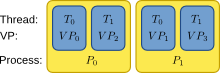Process_vp_thread Basic scheme for counting threads (T), virtual processes (VP) and MPI processes (P) in NEST

The status dictionary of each node (i.e. neuron or device) contains three entries that are related to parallel computing:

local (boolean): indicating if the node exists on the local process or not
thread (integer): id of the local thread the node is assigned to
vp (integer): id of the virtual process the node is assigned to.

Node distribution

The distribution of nodes is based on the type of the node. Neurons are assigned to one of the virtual processes in a round-robin fashion. On all other virtual processes, no object is created (the proxy object in the figure below is just a conceptual way of keeping the id of the real node free on remote processes). The virtual process id_VP on which a neuron with global id id_Node is allocated is given by id_VP = id_Node % N_VP, where N_VP is the total number of virtual processes in the simulation.

Devices for the stimulation and observation of the network are replicated once on each thread in order to balance the load of the different threads and minimize their interaction. Devices thus do not have proxies on remote virtual processes.

The node distribution for a small network consisting of spike_generator, four iaf_psc_alphas, and a spike_detector in a scenario with two processes with two threads each is shown in the following figure:

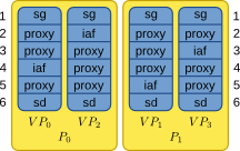Node_distribution Illustration of node distribution. sg=spike_generator, iaf=iaf_psc_alpha, sd=spike_detector. Numbers to the left and right indicate global ids.

For recording devices that are configured to record to a file (property to_file set to true), the distribution also results in multiple data files, each containing the data from one thread. The files names are composed according to the following scheme

[model|label]-gid-vp.[dat|gdf]

The first part is the name of the model (e.g. voltmeter or spike_detector) or, if set, the label of the recording device. The second part is the global id (GID) of the recording device. The third part is the id of the virtual process the recorder is assigned to, counted from 0. The extension is gdf for spike files and dat for analog recordings from the multimeter. The label and file_extension of a recording device can be set like any other parameter of a node using SetStatus.

Spike exchange and synapse updates

Spike exchange in NEST takes different routes depending on the type of the sending and receiving node. There are two distinct cases.

Spikes between neurons are always exchanged through the global spike exchange mechanism. Neuron update and spike generation in the source neuron and spike delivery to the target neuron may be handled by different virtual process in this case. Spike delivery is always handled by the virtual process to which the target neuron is assigned (see property vp in the status dictionary).

Spike exchange to or from neurons over connections that either originate or terminate at a device (e.g., spike_generator -> neuron or neuron -> spike_detector) differs in that it bypasses the global spike exchange mechanism. Instead, spikes are delivered locally within the virtual process from or to a replica of the device. In this case, both the pre- and postsynaptic nodes are handled by the virtual process to which the neuron is assigned.

For synapse models supporting plasticity, synapse dynamics in the Connection object are always handled by the virtual process of the target node.

Using multiple threads

Thread-parallelism is compiled into NEST by default and should work on all MacOS and Linux machines without additional requirements. In order to keep results comparable and reproducible across different machines, however, the default mode is that only a single thread is used and multi-threading has to be turned on explicitly.

To use multiple threads for the simulation, the desired number of threads has to be set before any nodes or connections are created. The command for this is

nest.SetKernelStatus({"local_num_threads": T})

Usually, a good choice for T is the number of processor cores available on your machine. In some situations, oversubscribing can yield 20-30% improvement in simulation speed. Finding the optimal thread number for a specific situation might require a bit of experimenting.

Using distributed computing

Build requirements

To compile NEST for distributed computing, you need a library implementation of MPI on your system. If you are on a cluster, you most likely have this already. Note, that in the case of a pre-packaged MPI library you will need both, the library and the development packages. Please see the Installation instructions for general information on installing NEST. Please be advised that NEST should currently only be run in a homogeneous MPI environment. Running in a heterogenenous environment can lead to unexpected results or even crashes. Please contact the NEST community if you require support for exotic setups.

Compilation

If the MPI library and header files are installed to the standard directories of the system, it is likely that a simple

$NEST_SOURCE_DIR/configure --with-mpi

will find them ($NEST_SOURCE_DIR is the directory holding the NEST sources). If MPI is installed to a non-standard location /path/to/mpi, the command line looks like this:

$NEST_SOURCE_DIR/configure --with-mpi=/path/to/mpi

In some cases it might be necessary to specify MPI compiler wrappers explicitly:

$NEST_SOURCE_DIR/configure CC=mpicc CXX=mpicxx --with-mpi

Additional information concerning MPI on OSX can be found here.

Running distributed simulations

Distributed simulations cannot be run interactively, which means that the simulation has to be provided as a script. However, the script does not have to be changed compared to the script for serial simulation: inter-process communication and node distribution is managed transparently inside of NEST.

To distribute a simulation onto 128 processes of a computer cluster, the command line to execute looks like this:

mpirun -np 128 python simulation.py

Please refer to the MPI library documentation for details on the usage of mpirun.

Although we generally advise strongly against writing process-aware code in simulation scripts (e.g. creating a neuron or device only on one process and such), in special cases it may be necessary to obtain information about the MPI application. One example would opening the right stimulus file for a specific rank. Therefore, some MPI specific commands are available:

NumProcesses
The number of MPI processes in the simulation

ProcessorName
The name of the machine. The result might differ on each process.

Rank
The rank of the MPI process. The result differs on each process.

SyncProcesses
Synchronize all MPI processes.

Reproducibility

To achieve the same simulation results even when using different parallelization strategies, the number of virtual processes has to be kept constant. A simulation with a specific number of virtual processes will always yield the same results, no matter how they are distributed over threads and processes, given that the seeds for the random number generators of the different virtual processes are the same (see Random numbers in NEST).

In order to achieve a constant number of virtual processes, NEST provides the property total_num_virtual_procs to adapt the number of local threads (property local_num_threads, explained above) to the number of available processes.

The following listing contains a complete simulation script (simulation.py) with four neurons connected in a chain. The first neuron receives random input from a poisson_generator and the spikes of all four neurons are recorded to files.

from nest import *
SetKernelStatus({"total_num_virtual_procs": 4})
pg = Create("poisson_generator", params={"rate": 50000.0})
n = Create("iaf_psc_alpha", 4)
sd = Create("spike_detector", params={"to_file": True})
Connect(pg, [n[0]], syn_spec={'weight': 1000.0, 'delay': 1.0})
Connect([n[0]], [n[1]], syn_spec={'weight': 1000.0, 'delay': 1.0})
Connect([n[1]], [n[2]], syn_spec={'weight': 1000.0, 'delay': 1.0})
Connect([n[2]], [n[3]], syn_spec={'weight': 1000.0, 'delay': 1.0})
Connect(n, sd)
Simulate(100.0)

The script is run three times using different numbers of MPI processes, but 4 virtual processes in every run:

mkdir 4vp_1p; cd 4vp_1p
mpirun -np 1 python ../simulation.py
cd ..; mkdir 4vp_2p; cd 4vp_2p
mpirun -np 2 python ../simulation.py
cd ..; mkdir 4vp_4p; cd 4vp_4p
mpirun -np 4 python ../simulation.py
cd ..
diff 4vp_1p 4vp_2p
diff 4vp_1p 4vp_4p

Each variant of the experiment produces four data files, one for each virtual process (spike_detector-6-0.gdf, spike_detector-6-1.gdf, spike_detector-6-2.gdf, and spike_detector-6-3.gdf). Using diff on the three data directories shows that they all contain the same spikes, which means that the simulation results are indeed the same independently of the details of parallelization.